Abstract
The quest for more efficient and faster deep learning models has led to the development of various alternatives to Transformers, one of which is the Mamba model. This paper provides a comprehensive comparison between Mamba models and Transformers, focusing on their architectural differences, performance metrics, and underlying mechanisms. It analyzes and synthesizes findings from extensive research conducted by various authors on these models. The synergy between Mamba models and the SciPy ecosystem enhances their integration into science. By providing an in-depth comparison using Python and its scientific ecosystem, this paper aims to clarify the strengths and weaknesses of Mamba models relative to Transformers. It offers the results obtained along with some thoughts on the possible ramifications for future research and applications in a range of academic and professional fields.
Introduction
The rapid advancements in deep learning have led to transformative breakthroughs across various domains, from natural language processing to computer vision. However, the quest for more efficient and scalable models remains a central challenge, especially when dealing with long sequences exhibiting long-range dependencies. Transformers, while achieving remarkable performance in numerous tasks, often suffer from high computational complexity and memory usage, particularly when handling long sequences.
This paper delves into the emerging field of State Space Models (SSMs) as a promising alternative to Transformers for efficiently capturing long-range dependencies in sequential data. We provide a comprehensive comparison between the recently developed Mamba model, based on SSMs, and the widely adopted Transformer architecture, highlighting their architectural differences, performance characteristics, and underlying mechanisms.
We begin by exploring the fundamental principles of SSMs, emphasizing their ability to represent and model continuous-time systems through a latent state vector. We then introduce the HiPPO framework, which extends SSMs to effectively handle long-range dependencies by leveraging the properties of orthogonal polynomials. This leads us to the discretization of continuous-time SSMs into discrete-time representations, enabling their implementation as recurrent models.
Building upon this foundation, we introduce the Structured State Space (S4) model, which addresses the computational limitations of traditional SSM implementations by employing a novel parameterization and efficient algorithms. S4’s Normal Plus Low-Rank (NPLR) decomposition allows for stable and efficient diagonalization of the state matrix, leading to significant improvements in computational complexity.
We then discuss the Mamba model, which leverages the selective SSM approach to capture long-range dependencies in sequences. The Mamba architecture combines aspects of RNNs, CNNs, and classical state space models, offering a unique blend of efficiency and expressivity.
The paper then presents a detailed comparison of Mamba and Transformer architectures, highlighting their core components, computational characteristics, and performance implications. We demonstrate the advantages of Mamba in terms of computational efficiency, memory usage, and sequence handling, underscoring its potential for tackling complex scientific and industrial problems.
Finally, we explore the potential applications and future directions of Mamba models, particularly in the context of scientific computing and data analysis. We highlight the synergy between Mamba and the SciPy ecosystem, underscoring its ability to enhance the efficiency and scalability of scientific computing workflows and drive novel scientific discoveries.
State Space Models
The central goal of machine learning is to develop models capable of efficiently processing sequential data across a range of modalities and tasks Albert Gu, Tri Dao, 2024. This is particularly challenging when dealing with long sequences, especially those exhibiting long-range dependencies (LRDs) – where information from distant past time steps significantly influences the current state or future predictions. Examples of such sequences abound in real-world applications, including speech, video, medical, time series, and natural language. However, traditional models struggle to effectively handle such long sequences.
Recurrent Neural Networks (RNNs) Sherstinsky, 2020, often considered the natural choice for sequential data, are inherently stateful and require only constant computation per time step. However, they are slow to train and suffer from the well-known “vanishing gradient problem”, which limits their ability to capture LRDs. Convolutional Neural Networks (CNNs) O'Shea & Nash, 2015, while efficient for parallelizable training, are not inherently sequential and struggle with long context lengths, resulting in more expensive inference. Transformers Vaswani et al., 2023, despite their recent success in various tasks, typically require specialized architectures and attention mechanisms to handle LRDs, which significantly increase computational complexity and memory usage.
A promising alternative for tackling LRDs in long sequences is State Space Models (SSMs) Gu et al., 2022, a foundational mathematical framework deeply rooted in diverse scientific disciplines like control theory and computational neuroscience. SSMs provide a continuous-time representation of a system’s state and evolution, offering a powerful paradigm for capturing LRDs. They represent a system’s behavior in terms of its internal state and how this state evolves over time. SSMs are widely used in various fields, including control theory, signal processing, and computational neuroscience.
Continuous-time Representation
The continuous-time SSM describes a system’s evolution using differential equations. It maps a continuous-time input signal to an output signal through a latent state . The state is an internal representation that captures the system’s history and influences its future behavior.
The core equations of the continuous-time SSM are:
State Evolution:
Output Generation:
where:
- is the state vector at time , belonging to a -dimensional space.
- is the input signal at time .
- is the output signal at time .
- is the state matrix, controlling the evolution of the state vector .
- is the control matrix, mapping the input signal to the state space.
- is the output matrix, projecting the state vector onto the output space.
- is the command matrix, directly mapping the input signal to the output. (For simplicity, we often assume = 0, as can be viewed as a skip connection.)
This system of equations defines a continuous-time mapping from input to output through a latent state . The state matrix plays a crucial role in determining the dynamics of the system and its ability to capture long-range dependencies.
HiPPO Framework for Long-Range Dependencies
Despite their theoretical elegance, naive applications of SSMs often struggle with long sequences. This is due to the inherent limitations of simple linear differential equations in capturing long-range dependencies (LRDs). To overcome this, the High-Order Polynomial Projection Operator (HiPPO) Gu et al., 2020 framework provides a principled approach for designing SSMs specifically suited for LRDs.
HiPPO focuses on finding specific state matrices that allow the state vector to effectively memorize the history of the input signal . It achieves this by leveraging the properties of orthogonal polynomials. The HiPPO framework derives several structured state matrices, including:
- HiPPO-LegT (Translated Legendre): Based on Legendre polynomials, this matrix enables the state to capture the history of the input within sliding windows of a fixed size.
- HiPPO-LagT (Translated Laguerre): Based on Laguerre polynomials, this matrix allows the state to capture a weighted history of the input, where older information decays exponentially.
- HiPPO-LegS (Scaled Legendre): Based on Legendre polynomials, this matrix captures the history of the input with respect to a linearly decaying weight.
Discrete-time SSM: Recurrent Representation
To apply SSMs on discrete-time data sequences (, , ...), it’s necessary to discretize the continuous-time model. This involves converting the differential equations into difference equations, where the state and input are defined at discrete time steps. One common discretization method is the bilinear transform, also known as the Tustin method. This transform approximates the derivative by a weighted average of the state values at two consecutive time steps, introducing a step size δ that represents the time interval between samples.
SSMs Figure 1 typically require integration within a broader neural network architecture due to their limited inherent capabilities. From a high-level perspective, SSMs exhibit functional similarities to linear Recurrent Neural Networks (RNNs). Both architectures process sequential input tokens, transforming and combining the previous hidden state representation with the embedding of the current input. This iterative processing characteristic aligns SSMs with the sequential nature of RNNs.
SSMs have 4 sets of matrices and parameters to process the input namely
where:
Δ acts as a gating factor, selectively weighting the contribution of matrices and at each step. This allows the model to dynamically adjust the influence of past hidden states and current inputs.
represents the state transition matrix. When modulated by Δ, it governs the propagation of information from the previous hidden state to the current hidden state.
denotes the input matrix. After modulation by Δ, it determines how the current input is integrated into the hidden state.
serves as the output matrix. It maps the hidden state to the model’s output, effectively transforming the internal representations into a desired output space.

Figure 1:This diagram illustrates the architecture of the Selective State Space Model (SSM). Each input sequence (blue boxes) is processed by an SSM layer (green) after being multiplied by matrix . The state space module (SSM) handles sequential data and captures long-range dependencies, after which the output (yellow boxes) undergoes a transformation by matrix . The final outputs (red boxes) are combined to produce the model’s output . This setup emphasizes the modular and repetitive nature of SSM layers, highlighting their role in sequence modeling.
The discretization technique facilitates the transformation of continuous differential equations into discrete time-step representations, leveraging the Δ matrix to decompose the infinitely continuous process into a discrete time-stepped process, thereby reducing computational complexity. In this approach, the and steps undergo discretization through the following equations:
This discretization scheme effectively reduces the continuous differential equation to a series of discrete time steps, enabling numerical approximations to be computed iteratively. By segmenting the continuous process into finite increments, the computational burden is alleviated, rendering the problem more tractable for numerical analysis and simulation.
Training SSMs
While the recurrent representation provides a computationally efficient way to perform inference with an SSM, it is not optimal for training due to its sequential nature. To overcome this, SSM leverages the connections between linear time-invariant (LTI) SSMs and convolution. The convolutional representation allows for efficient parallel training using Fast Fourier Transform (FFT) algorithms. However, the main challenge lies in computing the SSM convolution kernel . Computing it naively with successive matrix multiplications by results in operations and memory – a significant computational bottleneck for long sequences.
The state-space models (SSMs) compute the output using a linear recurrent neural network (RNN) architecture, which operates on a hidden state Δ. In this formulation, the hidden state propagates through a linear equation of the following form:
where
- is hidden state matrix at time step t
- is input vector at time t
The initial hidden state is computed as:
Subsequently, the hidden state at the next time step, , is obtained through the recursion:
The output is then calculated from the hidden state using the following linear transformation:
- C is the output control matrix
- is output vector at time t
- is the Internal hidden state at time t
where :
- is the input matrix i.e.
This linear RNN architecture effectively captures the temporal relationships present in sequential data and thus enabling the model to learn and ensure the propagation of the key-relevant information through the recurrent connections. This linear formulation has led to scalable implementations, which in turn take use of matrix operations’ computing efficiency.
S4: A Structured State Space Model
The theoretical advantages of State Space Models (SSMs) Gu et al., 2022 for handling long sequences, particularly their ability to capture long-range dependencies, make them a promising alternative to traditional sequence models. However, the computational limitations of existing SSM implementations, such as the LSSL, hinder their widespread adoption. The Structured State Space (S4) model aims to overcome these limitations by introducing novel parameterization Gu et al., 2022 and efficient algorithms that preserve the theoretical strengths of SSMs Albert Gu, Karan Goel, Christopher Ré, 2021 .
Diagonalization Problem
The core computational bottleneck in SSMs stems from repeated matrix multiplication by the state matrix when calculating the convolution kernel . If were a diagonal matrix, this computation would become significantly more tractable. Diagonal matrices allow for efficient power calculations as well as multiplication by a vector, resulting in a time complexity of for dimensions.
Diagonalization involves finding a change of basis that transforms into a diagonal form. However, this approach faces significant challenges when is non-normal. Non-normal matrices have complex eigenstructures, which can lead to several problems:
- Numerically unstable diagonalization: Diagonalizing non-normal matrices can be numerically unstable, especially for large matrices. This is because the eigenvectors may be highly sensitive to small errors in the matrix, leading to large errors in the computed eigenvalues and eigenvectors.
- Exponentially large entries: The diagonalization of some non-normal matrices, including the HiPPO matrices, can involve matrices with entries that grow exponentially with the dimension . This can lead to overflow issues during computation and render the diagonalization infeasible in practice.
Therefore, naive diagonalization of non-normal matrices in SSMs is not a viable solution for efficient computation.
The S4 Parameterization: Normal Plus Low-Rank (NPLR)
S4 overcomes the challenges of directly diagonalizing non-normal matrices by introducing a novel parameterization Gu et al., 2022. It decomposes the state matrix A into a sum of a normal matrix and a low-rank term. This decomposition allows for efficient computation while preserving the structure necessary to handle long-range dependencies. The S4 parameterization is expressed as follows:
- SSM convolution kernel
where:
- V is a unitary matrix that diagonalizes the normal matrix.
- Λ is a diagonal matrix containing the eigenvalues of the normal matrix.
- P and Q are low-rank matrices that capture the non-normal component.
- These matrices HiPPO - all satisfy = 1 or = 2.
This decomposition allows for efficient computation because:
- Normal matrices are efficiently diagonalizable: Normal matrices can be diagonalized stably and efficiently using unitary transformations.
- Low-rank corrections are tractable: The low-rank term can be corrected using the Woodbury identity, a powerful tool for inverting matrices perturbed by low-rank terms.
S4 Algorithms and Complexity
S4 leverages its NPLR parameterization to develop efficient algorithms for computing both the recurrent representation () and the convolutional kernel ().
S4 Recurrence
The bilinear transform is used to discretize the state matrix in order to construct the S4 recurrent representation. The important thing to note is that, because of the Woodbury identity, the inverse of a DPLR matrix does not result in any change in the matrix. Therefore, the discretized state matrix is the product of two DPLR matrices, allowing for efficient matrix-vector multiplication in O(N) time.
Parallel Associative Scan
The linear recurrent behavior inherent in the previous formulation is not efficiently implementable on GPU architectures, which favor parallel computing paradigms. This limitation renders convolutions inefficient in such environments. To address this challenge, the parallel associative scan technique is employed, which introduces a prefix sum-like operation to scan for all prefix sums. Although inherently sequential, this approach leverages an efficient parallel algorithm model to parallelize the SSM convolution, resulting in a significant performance boost. The parallel associative scan method exhibits linear time and space complexity, making it a computationally efficient solution.
SSM
Selective SSM
By leveraging the parallel associative scan technique Lim et al., 2024, the selective SSM formulation can be efficiently implemented on parallel architectures, such as GPUs. This approach enables the exploitation of the inherent parallelism in the computation, leading to significant performance gains, particularly for large-scale applications and time-series data processing tasks.
S4 Convolution
S4’s convolutional representation is computed through a series of steps:
- SSM Generating Function: Instead of directly computing the convolution kernel , S4 calculates its spectrum by evaluating its truncated generating function. The generating function allows for efficiently expressing powers of as a single matrix inverse.
- Woodbury Correction: The Woodbury identity is used to correct the low-rank term in the generating function, reducing the problem to evaluating the generating function for a diagonal matrix.
- Cauchy Kernel: The generating function for a diagonal matrix is equivalent to computing a Cauchy kernel, which is a well-studied problem with efficient, numerically stable algorithms.
This process reduces the complexity of computing the convolution kernel to operations and memory, significantly improving upon the LSSL’s complexity.
S4 Architecture Details
The S4 layer, as defined by its NPLR parameterization, implements a mapping from a 1-D input sequence to a 1-D output sequence. To handle multiple features, the S4 architecture utilizes independent copies of the S4 layer, each processing one feature dimension. These outputs are then mixed using a position-wise linear layer, similar to a depthwise-separable convolution. This architecture allows for efficient computation while preserving the ability to capture relationships between different features.
Non-linear activation functions are typically added between S4 layers to enhance the model’s expressivity, further paralleling the structure of CNNs. Thus, the overall deep S4 model resembles a depthwise-separable CNN, but with global convolution kernels that effectively capture long-range dependencies.
In summary, S4 offers a structured and efficient approach to SSMs, overcoming the limitations of previous implementations while preserving their theoretical strengths. Its NPLR parameterization allows for stable and efficient computation, while its efficient algorithms significantly reduce computational complexity. S4’s ability to handle multiple features and its resemblance to CNNs further contribute to its versatility and potential as a powerful general sequence modeling solution.
Mamba Model Architecture
One Mamba Layer Gu & Dao, 2023 Figure 2 is composed of a selective state-space module and several auxiliary layers. Initially, a linear layer doubles the dimensionality of the input token embedding, increasing the dimensionality from 64 to 128. This higher dimensionality provides the network with an expanded representational space, potentially enabling the separation of previously inseparable classes. Subsequently, a canonical 1D convolution layer processes the output of the previous layer, manipulating the dimensions within the linearly upscaled 128-dimensional vector. This convolution layer employs the SiLU (Sigmoid-weighted Linear Unit) activation function Elfwing et al., 2017. The output of the convolution is then processed by the selective state-space module, which operates akin to a linear recurrent neural network (RNN).

Figure 2:This diagram represents the Mamba architecture, illustrating the flow from input through convolutional and sequence transformation layers, with nonlinear activation functions, to produce the final output via linear projection.
Mamba then performs a gated multiplication operation. The input is passed through another linear layer and an activation function, and the resulting output is multiplied element-wise with the output of the S4 module. The authors’ intuition behind this operation is that the multiplication serves as a measure of similarity between the output of the SSM module, which contains information from previous tokens, and the embedding of the current token. Finally, a linear layer reduces the dimensionality from 128 back to 64. To construct the complete Mamba architecture, multiple layers are stacked on top of one another, similar to the Transformer architecture, where Transformer layers are stacked sequentially.
Key Differences Between Mamba and Transformer Architectures
In this section, we present a detailed comparison of the Mamba and Transformer architectures. We focus on their core components, computational characteristics, and performance implications. Visualizations and equations are provided to illustrate these differences clearly.
Self attention, feed forward Neural Networks, normalization, residual layers and so on.
Architecture Overview
Transformer Architecture
Transformers Figure 3 rely heavily on attention mechanisms to model dependencies between input and output sequences. A better understanding of the code will be of great helpAshish Vaswani, Noam Shazeer, Niki Parmar, Jakob Uszkoreit, Llion Jones, Aidan N. Gomez, Lukasz Kaiser, Illia Polosukhin, 2017.
The core components include:
- Multi-Head Self-Attention: Allows the model to focus on different parts of the input sequence.
- Position-wise Feed-Forward Networks: Applied to each position separately.
- Positional Encoding: Adds information about the position of each token in the sequence, as Transformers lack inherent sequential information due to the parallel nature of their processing.
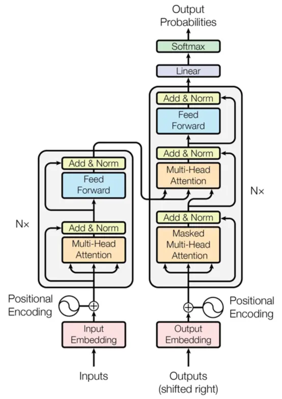
Figure 3:This diagram illustrates the transformer model architecture, featuring encoder and decoder layers with multi-head attention mechanisms, positional encoding, and feed-forward networks, culminating in output probabilities via a softmax layer.
Mamba Architecture
Mamba models Figure 2 are based on Selective State Space Models (SSMs), combining aspects of RNNs, CNNs, and classical state space models. Key features include:
- Selective State Space Models: Allow input-dependent parameterization to selectively propagate or forget information.
- Recurrent Mode: Efficient recurrent computations with linear scaling.
- Hardware-aware Algorithm: Optimized for modern hardware to avoid inefficiencies from the Flash Attention 2 Paper. [@]
Key Differences
1. Attention Mechanisms vs. Selective State Space Models
Transformers use multi-head self-attention to capture dependencies within the sequence:
Where , , and are the query, key, and value matrices, respectively, and is the dimension of the key vectors.
Mamba Models replace attention with selective state space parameters that change based on the input:
Here, , , and are state space parameters that vary with the input, allowing for efficient handling of long sequences without the quadratic complexity of attention mechanisms.
2. Computational Complexity
| Feature | Architecture | Complexity | Inference Speed | Training Speed |
|---|---|---|---|---|
| Transformer | Attention-based | High | O(n) | O(n²) |
| Mamba | SSM-based | Lower | O(1) | O(n) |
3. Sequence Handling and Memory Efficiency
Transformers require a cache of previous elements to handle long-range dependencies, leading to high memory usage.
Mamba Models utilize selective state spaces to maintain relevant information over long sequences without the need for extensive memory caches, providing a more memory-efficient solution.
Mamba integrates selective state spaces directly into the neural network architecture. The selective mechanism allows the model to focus on relevant parts of the input dynamically.
There are other competing architectures that aim to replace or complement Transformers, such as Retentive Network Sun et al., 2023, Griffin De et al., 2024, Hyena Poli et al., 2023, and RWKV Peng et al., 2023. These architectures propose alternative approaches to modeling sequential data, leveraging techniques like gated linear recurrences, local attention, and reinventing recurrent neural networks (RNNs) for the Transformer era.
Mamba’s Synergy with Scipy
Scipy Virtanen et al., 2020 provides a robust ecosystem for scientific computing in Python, offering a wide range of tools and libraries for numerical analysis, signal processing, optimization, and more. This ecosystem serves as a fertile ground for the development and integration of Mamba, facilitating its training, evaluation, and deployment in scientific applications. Leveraging Scipy’s powerful data manipulation and visualization capabilities, Mamba models can be seamlessly integrated into scientific workflows, enabling in-depth analysis, rigorous statistical testing, and clear visualization of results.
The combination of Mamba’s language understanding capabilities and Scipy’s scientific computing tools opens up new avenues for exploring large-scale scientific datasets commonly encountered in scientific research domains such as astronomy, medicine, and beyond, extracting insights, and advancing scientific discoveries.
Potential Applications and Future Directions:
- Efficient Processing of Large Scientific Datasets: Mamba’s ability to handle long-range dependencies makes it well-suited for analyzing and summarizing vast amounts of scientific data, such as astronomical observations, medical records, or experimental results, thereby reducing the complexity and enabling more efficient analysis.
- Enhancing Model Efficiency and Scalability: Integrating Mamba with Scipy’s optimization and parallelization techniques can potentially improve the efficiency and scalability of language models, enabling them to handle increasingly larger datasets and more complex scientific problems.
- Advancing Scientific Computing through Interdisciplinary Collaboration: The synergy between Mamba and Scipy fosters interdisciplinary collaboration between natural language processing researchers, scientific computing experts, and domain-specific scientists, paving the way for novel applications and pushing the boundaries of scientific computing.
The diverse range of models as U-Mamba Ma et al., 2024, Vision MambaZhu et al., 2024, VMamba Liu et al., 2024, MambaByte Wang et al., 2024and Jamba Lieber et al., 2024, highlights the versatility and adaptability of the Mamba architecture. These variants have been designed to enhance efficiency, improve long-range dependency modeling, incorporate visual representations, explore token-free approaches, integrate Fourier learning, and hybridize with Transformer components.
Conclusion
Mamba models present a compelling alternative to Transformers for processing long sequences, particularly in scientific computing. Their use of selective state spaces delivers linear time complexity and superior memory efficiency, making them faster and less resource-intensive than Transformers for lengthy data. Mamba’s flexible architecture enables easy integration with scientific workflows and scalability. However, their complexity demands further research to streamline implementation and encourage wider adoption. While not yet a complete replacement for Transformers, Mamba models offer a powerful tool for analyzing complex scientific data where efficiency and integration with scientific tools are paramount, making their continued development crucial.
- Albert Gu, Tri Dao. (2024). Mamba: Linear-Time Sequence Modeling with Selective State Spaces. https://github.com/state-spaces/mamba
- Sherstinsky, A. (2020). Fundamentals of Recurrent Neural Network (RNN) and Long Short-Term Memory (LSTM) network. Physica D: Nonlinear Phenomena, 404, 132306. 10.1016/j.physd.2019.132306
- O’Shea, K., & Nash, R. (2015). An Introduction to Convolutional Neural Networks. https://doi.org/10.48550/arXiv.1511.08458
- Vaswani, A., Shazeer, N., Parmar, N., Uszkoreit, J., Jones, L., Gomez, A. N., Kaiser, L., & Polosukhin, I. (2023). Attention Is All You Need. https://doi.org/10.48550/arXiv.1706.03762
- Gu, A., Goel, K., & Ré, C. (2022). Efficiently Modeling Long Sequences with Structured State Spaces. https://doi.org/10.48550/arXiv.2111.00396